Posted July 30, 2020

I was playing the original Yoshi's Island (well, technically the GBA remake, but potato potahto), and I encountered the roulette minigame. I thought it would be particularly fun to massively overanalyze the minigame, as there's potential for some interesting statistical calculations to be done.

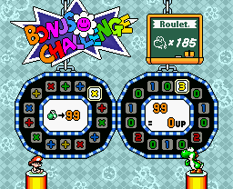
This is the game I'm talking about. First, you bet any number of lives, from 1 to 99. Then you spin both of the wheels above to form, essentially, a math equation. So if I were to bet 45 lives, then the wheels landed on "\(+ 3\)", I'd get \(45 + 3 = 48\) lives. If they landed on "\(\times 2\)", I'd get \(45 \times 2 = 90\) lives. The game isn't an auto-win. A "\(\times 0\)" result means you lose whatever lives you put in, so there's definitely a real possibility of losing. So the question is: if I bet \(N\) lives, what's the expected return?

I'm going to analyze this from a few different angles. First, we're going to simply get the answer the quick-and-dirty way. Then we'll see how far down the rabbit hole we can take this and have some fun with linear algebra. Also, I'll be making a few common sense assumptions. I haven't delved into the game's code to see if this is true or not, but I'm assuming that the wheel has a uniform probability of stopping on any given position, i.e. that the game isn't rigged. I'm also assuming that the two wheels are statistically independent events. The latter assumption may not be true, since the wheels do start spinning at the same time, so theoretically (especially if you stop them quickly) they may be tied together, but we won't be considering that possibility here.

So, step one is to get our answer. The "\(+\)" outcomes are less interesting, because their expected value doesn't depend on my input. Regardless of how many lives I wager, a "\(+ 2\)" result has a value of 2. So, for a cursory analysis, "\(+\)" is going to have a constant expected value, regardless of my input value. The "\(\times\)" cases are more interesting. A "\(\times 1\)" result simply means I get my original wager back, so I gained nothing. That is, "\(\times 1\)" has an expected value of zero. In general, if I wager \(N\) lives and land on "\(\times k\)", then the return is \((k-1)N\). The outcomes in the roulette also aren't equinumerous. That is, there's only one "3" in the wheel, but there are several "0"s. The table below summarizes the appearance rates and expected values of the numbers, assuming we land on "\(\times\)".

Outcome	Probability	Expected Value
0	50.0%	\(-N\)
1	28.6%	\(0\)
2	14.2%	\(N\)
2	7.1%	\(2 N\)

Now, the (discrete) expected value is simply the sum of each outcome times its likelihood. So

$$E[X \mid L = \times] = 0.500 (- N) + 0.286 (0) + 0.142 N + 0.071 (2 N) = -0.216 N$$

So multiplication is a loss. If we get a "\(\times\)" on the left wheel, we should expect to lose 21.6% of what we put in. Naturally, since the expected value is negative and proportional to our input, it makes sense that we should minimize the number of lives we put in. So if we're going to play the roulette, we should wager one life, to minimize our losses on the "\(\times\)" outcome.

But the next logical question is: should we play at all? That is, is there a positive overall expected value from wagering one life, or should we just exit the minigame entirely to get a surefire expected value of zero? Well, we know the expected value of the "\(\times\)" outcome, and we can modify the above table to work for the "\(+\)" outcome. Assuming the left wheel lands on "\(+\)", the possible results are as follows.

Outcome	Probability	Expected Value
0	50.0%	\(0\)
1	28.6%	\(1\)
2	14.2%	\(2\)
2	7.1%	\(3\)

And our calculation is

$$E[X \mid L = +] = 0.500 (0) + 0.286 (1) + 0.142 (2) + 0.071 (3) = 0.783$$

Naturally, the expected value is positive, since we stand to lose nothing if we land on "\(+\)". Now, if we look at the left wheel, "\(+\)" appears 8 times while "\(\times\)" appears 6. So there's a 57.1% chance of getting "\(+\)" and a 42.9% chance of getting "\(\times\)".

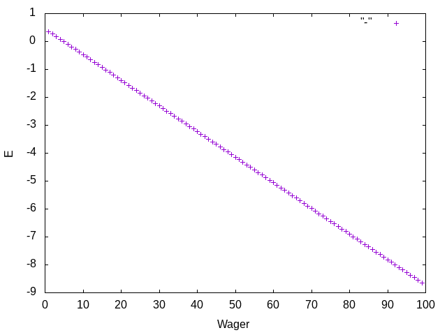
$$E[X] = 0.571 \times E[X \mid L = +] + 0.428 \times E[X \mid L = \times] = 0.571 \times 0.783 + 0.428 \times (-0.216 N) = 0.447 - 0.092 N$$

And there's the general formula for the expected value of lives gained or lost, given an initial wager of \(N\). It's linear with a negative slope, and it crosses zero at \(N = 4.86\). So, as we found before, the optimal play is to wager one life. As long as you wager between one and four lives, your expected value is still positive. Wagering five or more lives will, on average, result in a loss, because the "\(\times 0\)" outcome becomes much more dangerous, the more you wager.

Okay, we have our answer. Neat. We're done here, right? Well, no, not exactly. We did all of these calculations by hand. Which is fine given that each roulette wheel has 14 slots, and there's really only 8 possible results from the roulette game anyway. But let's talk a bit more about the mathematics behind this and about how we would solve this abstractly, in a way that would apply to, say, a 1,000-slot roulette wheel with 200 outcomes, where we really, really don't want to do everything by hand.

I'll be using APL for the calculations here, and we'll see if we can get our original result back using the computer. Specifically, I'll be using ngn APL, which can be installed from the Node package manager. So let's get started. First off, APL is array-based. So the more linear we can make this problem, the easier it's going to get. Representing the multiplications (i.e. the "\(\times\)" on the left wheel) as linear transformations is easy: linear transformations in one-dimension are exactly multiplications. The "\(+\)" outcome poses a bit more of a challenge. Adding a constant value is not, by itself, a linear map. But it can be made into one, with some concessions.

This particular problem has cropped up before, specifically in computer graphics. Most standard transformation operations (reflections and rotations, in particular) can be nicely represented as matrices, which is great. But the issue comes when we try to make a translation into a matrix. At a glance, there's no way to encode the action "move this picture ten units to the left" as a matrix.

But there's a solution. A translation is linear, in an argument we can't see. Rather than dealing with just three coordinates (X, Y, and Z), we add a fourth coordinate which is always 1. Then our transformation matrices are no longer 3×3 but instead are 4×4. In order to maintain the invariant that the fourth coordinate is always 1, we require that the bottom row of our matrix be \(\begin{bmatrix}0&0&0&1\end{bmatrix}\). But that still give us three new entries to manipulate in our matrix (the rightmost column), and in fact those three entries correspond directly to X, Y, and Z translations, respectively.

We do lose a bit of the niceness of linear algebra with this hack. When we've done our calculations, we need to "normalize" our resulting vector so that the fourth coordinate is 1 again. This can easily get off if we end up multiplying a transformation matrix by a scalar at some point, which is a pretty common operation, or if we end up adding two matrices. So it's just worth keeping in mind that we may have to scale our vector down at the end.

But we can still use this solution for our roulette problem as well. Our input wager and expected value are both 1-dimensional values (really, they're scalars, but up to isomorphism we can pretend they're vectors). So we'll add in an extra dimension which is always 1 as an additive term. So, for instance, our "\(\times 2\)" outcome in the roulette leaves the additive term alone and just multiplies by 2. That corresponds to the matrix

$$\begin{bmatrix}2 & 0 \\ 0 & 1\end{bmatrix}$$

Addition is done by multiplying the wager by 1 (since we get the original wager back), then adding a constant amount. So, for instance, "\(+ 2\)" would be represented by

$$\begin{bmatrix}1 & 2 \\ 0 & 1\end{bmatrix}$$

But we're doing this abstractly. We could take it one step further. The general forms "\(\times k\)" and "\(+k\)" are represented, respectively, by

$$\begin{bmatrix}k & 0 \\ 0 & 1\end{bmatrix}, \begin{bmatrix}1 & k \\ 0 & 1\end{bmatrix}$$

The first matrix, given an input as a 2-vector with second coordinate 1, will multiply by \(k\). The second, likewise, will add \(k\) to the input value. The next question is: can we generalize it? Can we produce some pair of operations that, given an input value, produces the above matrices? Let's focus on multiplication for the moment, and then we'll come back to addition.

I want an operation that, given an integer, produces a particular matrix. That matrix should have our input integer in the top-left, a constant 1 in the bottom-right, and zeroes elsewhere. That is, I want a map from \(\mathbb{Z}\) to \(\mathbb{Z}^{2 \times 2}\). Again, we'll consider \(\mathbb{Z}\), up to isomorphism, as a one-dimensional module over itself.

Now, we're already far enough down this rabbit hole, so let's go all the way. In full generality, matrices and vectors are just part of a larger hierarchy of tensors of any rank. Now, you can read tons of mathematical literature on tensors, but for me it never really clicked until I started using them in APL and similar languages. So I'll approach the problem like an APL programmer, because that's what worked for me when figuring all of this stuff out. Higher-ranked tensors arise naturally when noting that vectors are really a thing where we can refer to a position by one coordinate, whereas in a matrix we really need two coordinates to refer to a position. It may be tempting to refer to this as the "dimension" of the tensor, but I'm deliberately avoiding that term as "dimension" is referring to a different property of the space.

If we have a scalar, we have only one thing. There's no need for coordinates at all. If I give you a scalar and ask you what number it is, you really don't need any more information. Hence, we need zero coordinates. A scalar is a rank 0 tensor. If I have a vector, I can show it to you, give you a single coordinate, and ask what number appears at that position. Hence, vectors are rank 1 tensors. If I have a matrix, it'll take two coordinates to specify a position containing a single value. So matrices are rank 2 tensors. The rank simply corresponds to how much information I have to give you to get at the actual data. We don't really have names for tensors of rank higher than 2, so we'll generally just say "rank 3 tensor", etc.

Another bit of terminology that will come in handy later is to discuss a tensor's shape. Just as a matrix has a shape, in some sense (we might say a matrix has shape \(2 \times 2\)), all tensors really have a shape in the same sense. The shape of a vector is simply the number of elements in it. The shape of a scalar is empty, since it has no coordinates (crucially, it's not zero; a tensor with shape zero is an empty vector, not a scalar). The shape of a matrix is its width and height. The shape of a rank 3 tensor would be three numbers specifying its width, height, and... length, I suppose. In general, the rank of a tensor is the dimension (i.e. length of the vector) of its shape. For higher rank tensors, I'll use row vector notation to talk about their shape, so rather than say a tensor has shape \(2 \times 2 \times 2\), I would say it has shape \(\begin{bmatrix} 2 & 2 & 2 \end{bmatrix}\).

How does any of this apply to anything we've done? Good question. Earlier, we had a map from vectors to vectors (the "\(+2\)" map, for instance). That map was realized as a matrix. Said once again, we had a map from rank 1 tensors to rank 1 tensors, and we realized it as a rank 2 tensor. Written using obtuse mathematical jargon, that corresponds to the following well-known isomorphism in linear algebra (assuming the relevant modules are finite-dimensional).

$$\mathscr{L}(V, W) \cong V^* \otimes_{A} W \cong V \otimes_{A} W$$

Note that, if you're not mathematically inclined, you can pretend those \(\cong\) are equal signs. In particular, they don't mean "approximately" as they do in some scientific fields. The \(\cong\) symbol, here, means "isomorphic", which is a subtle concept weaker than equality but still retaining many of its nice properties. If you don't have a background in category theory, it should be pretty safe, for the duration of this post at least, to pretend they're just equal signs.

\(\mathscr{L}(V, W)\) is the space of linear maps from \(V\) to \(W\), under pointwise addition and scalar multiplication. \(V^*\) is the dual module of \(V\), which in the finite-dimensional case is isomorphic (though not naturally so) to \(V\) itself. Finally, \(\otimes_{A}\) is the tensor product over our scalar ring \(A\). In particular, if \(V = A^n, W = A^m\) are both finite-dimensional free modules over the same ring, then \(A^n \otimes_A A^m \cong A^{n \times m}\). The tensor product is really just the space of matrices. You can add a bunch of dense mathematics to it all and talk about universal properties all you want, but for a beginning understanding this is all it is. All I've said with this equation is exactly what I said before: linear maps which takes vectors to vectors can be realized as matrices.

But we said we wanted a map which takes a vector to a matrix. We're operating over the integers, so we want to ask what \(\mathscr{L}(\mathbb{Z}^2, \mathbb{Z}^{2 \times 2})\) looks like (Note that we're assuming our input is 2-dimensional again; since we want to eventually encode addition, we may as well go ahead and add in our additive term that's always 1 like before). Let's apply the same isomorphism as before.

$$\mathscr{L}(\mathbb{Z}^2, \mathbb{Z}^{2 \times 2}) \cong (\mathbb{Z}^2)^* \otimes (\mathbb{Z}^{2 \times 2}) \cong \mathbb{Z}^2 \otimes \mathbb{Z}^{2 \times 2} \cong \mathbb{Z}^2 \otimes \mathbb{Z}^2 \otimes \mathbb{Z}^2$$

So a map from vectors to matrices can be realized as a rank 3 tensor, specifically a rank 3 tensor with shape \(\begin{bmatrix} 2&2&2 \end{bmatrix}\). When we did the additive hack with matrices before, we needed the entire bottom row to be zeroes followed by a single one. Now, we don't have a bottom "row", we have an entire bottom matrix, which will have to be zeroes with a single one in the lower-right corner. We're talking about multiplication first, so we want an input of \(k\) to this rank 3 tensor to give us an output of

$$\begin{bmatrix}k & 0 \\ 0 & 1\end{bmatrix}$$

I don't know the best way to represent rank 3 tensors in three actual dimensions in this post, so I'll represent them as two matrices next to each other. We want the first entry to be inserted in the top-left corner, and the top-right term should be zero. Hence, we want

$$\begin{bmatrix}1 & 0 \\ 0 & 0\end{bmatrix} \begin{bmatrix}0 & 0 \\ 0 & 1\end{bmatrix}$$

That's multiplication. Now, in the case of addition, we want an input of \(k\) to produce the matrix

$$\begin{bmatrix}1 & k \\ 0 & 1\end{bmatrix}$$

So we want to put \(k\) at the top-right position and a constant (i.e. additive) 1 at the top-left. We want

$$\begin{bmatrix}0 & 1 \\ 1 & 0\end{bmatrix} \begin{bmatrix}0 & 0 \\ 0 & 1\end{bmatrix}$$

Don't worry if you don't fully grok the order of indices or why I put ones where I did. Coordinates are easy to confuse, and it took me three or four tries to get that right anyway. The important thing is there's three ones in that matrix. The lower-right one is required and doesn't tell us anything, and the other two are because we're doing two "things": putting a \(k\) somewhere and putting a 1 somewhere else.

Just for the sake of completeness (we won't need this for the rest of this post), we can also represent subtraction as follows

$$\begin{bmatrix}0 & 1 \\ -1 & 0\end{bmatrix} \begin{bmatrix}0 & 0 \\ 0 & 1\end{bmatrix}$$

Swapping the left -1 and 1 would reverse the order of subtraction (i.e. one computes \(\cdot-k\) where the other computes \(k-\cdot\)). That didn't come into play with addition and multiplication since both are commutative. Division is... trickier, since it's not a linear map, and it's going to be very difficult to realize as a linear map, even with our hack. I don't offhand know how to realize it as a tensor, but fortunately we don't need it right now. So we now have high-rank tensors that represent the basic mathematical operations of \(+\) and \(\times\) (and \(-\), but like I said that doesn't pertain to the roulette game).

But how do we multiply these? A better first question would be: how do we multiply matrices? Seriously, think about it. When I think about matrix multiplication, I do a funny gesture with my hand involving sliding a row along a column of an invisible matrix I'm imagining in the air. It's not very mathematical. Before reading on, try to explain mathematically what matrix multiplication actually is. I'm sure you can, but it may not come as quickly as you might've thought.

Matrix multiplication is an operation we can perform to take an \(n \times m\) matrix and an \(m \times k\) matrix and produce an \(n \times k\) matrix. Note that the last coordinate of the first matrix must match the first coordinate of the last matrix. This will remain important in our generalization. In our result matrix, the \((i, k)\) term sums over all possible values of the middle coordinate. So if \(C = AB\), then we have

$$c_{ik} = \sum_j a_{ij} b_{jk}$$

And now we can generalize. If we have two tensors, one with shape \(\begin{bmatrix}i_1 & i_2 & \dots & i_n & j\end{bmatrix}\) and the other with shape \(\begin{bmatrix}j & k_1 & k_2 & \dots & k_m \end{bmatrix}\) (Note, crucially, that the last coordinate of the first and the first coordinate of the last still line up), then we can meaningfully multiply them to get a tensor with shape \(\begin{bmatrix}i_1 & i_2 \dots & i_n & k_1 & k_2 & \dots & k_m \end{bmatrix}\) as follows. If \(C = AB\) using the same notation as before, then

$$c_{i_1 \dots i_n k_1 \dots k_m} = \sum_j a_{i_1 \dots i_n j} b_{j k_1 \dots k_m}$$

What does this mean mathematically? Well, really, it's just an application of the evaluation map. Remember, for finite dimensional free modules, a module is isomorphic to its dual. If you followed that dual link above, you learned that the dual module \(V^*\) is just the module of maps \(V \to A\) where \(A\) is the underlying ring. So if we have an element of \(V\) and an element of \(V^*\), we can combine them to get an element of \(A\) by simply applying the function to its argument. That is, we have a map

$$\mathrm{eval} : V \otimes_A V^* \to A$$

Why don't we define this from \(V \times V^*\)? Well, it's bilinear from \(V \times V^*\), which means (almost, but not quite, by definition) that it's linear from \(V \otimes_A V^*\). So this version of the evaluation map is a linear map, which is a nice property to have.

There are two other useful properties we'll need. First, there's a canonical bilinear map from the product to the tensor product, i.e. \(V \times W \to V \otimes W\). This ties into the universal property which defines the tensor product, but that's not important right now. Second, the tensor operation is actually monoidal, which is a fancy way of saying that it's (up to isomorphism, but again, that's not really the focus right now) associative and has an identity \(A\). So \(A \otimes V \cong V \otimes A \cong V\), provided \(A\) is the underlying scalar ring. Now we combine all this together. We start with tensors of respective shapes \(\begin{bmatrix}i_1 & i_2 & \dots & i_n & j\end{bmatrix}\) and \(\begin{bmatrix}j & k_1 & k_2 & \dots & k_m \end{bmatrix}\). That is, we start with an element of the direct product

$$(A^{i_1} \otimes \dots \otimes A^{i_n} \otimes A^j) \times (A^j \otimes A^{k_1} \otimes \dots \otimes A^{k_m})$$

We inject into the tensor product with the canonical bilinear map.

$$A^{i_1} \otimes \dots \otimes A^{i_n} \otimes A^j \otimes A^j \otimes A^{k_1} \otimes \dots \otimes A^{k_m}$$

Note that, up to isomorphism, the tensor product is associative, so I'll be omitting the parentheses. Next, we note that, since everything is finite-dimensional, \(A^j \cong (A^j)^*\), so we have

$$A^{i_1} \otimes \dots \otimes A^{i_n} \otimes A^j \otimes (A^j)^* \otimes A^{k_1} \otimes \dots \otimes A^{k_m}$$

Finally, we apply the evaluation map \(\mathrm{eval} : A^j \otimes (A^j)^* \to A\) to the inner tensor product. Why can we apply it to only one part of the tensor product? The tensor product is a functor in both arguments (that is, it's a bifunctor), which exactly tells us we can do this. So we get

$$A^{i_1} \otimes \dots \otimes A^{i_n} \otimes A \otimes A^{k_1} \otimes \dots \otimes A^{k_m}$$

Finally, \(A\) is the identity of the tensor product monoidal operation, so it has no effect. This gives us the shape we want.

$$A^{i_1} \otimes \dots \otimes A^{i_n} \otimes A^{k_1} \otimes \dots \otimes A^{k_m}$$

The good news is: we don't really need all this theory for the purposes of our program. APL's standard matrix multiplication operation is actually an incredibly general inner product operation that will just automatically do the thing we want it to. So we literally don't have to do anything different at all to get all this theory to work.

Okay, whew! That was a lot of theory. Now let's do some calculations. Time to write actual code. First, I'll define a helper function. We'll be using vectors to represent the probability states, and crucially a probability state should always have its probabilities sum to 1. So this function will normalize a vector to have sum (i.e. taxicab norm) 1.

norm←⊢÷(+/)
      

(Side note: I'm sorry for the lack of syntax highlighting here. My usual syntax highlighter doesn't support APL, sadly. I may end up writing it myself, but for now, enjoy the white text.)

This is a specific instance of a neat concept many APL dialects support called a verb train. We're defining a verb norm, and our train consists of three verbs ⊢ ÷ (+/). The way to read this is: take the input (⊢) and divide it (÷) by its sum (+/).

Next, we'll encode our \(+\) and \(\times\) tensors from above. lhsEffect consists of the two rank 3 tensors we discovered above, while lhsProb consists of their respective probabilities.

lhsEffect←(2 2 2⍴0 1 1 0 0 0 0 1)(2 2 2⍴1 0 0 0 0 0 0 1)
lhsProb←norm 8 6
      

Then the same for the right-hand roulette wheel: rhsEffect are the values and rhsProb are their probabilities.

rhsEffect←0 1 2 3
rhsProb←norm 7 4 2 1
      

We also need to note that, before starting, we lose our wager, which puts us at a disadvantage (it wouldn't be much of a gamble if we didn't, well, gamble anything).

wager←2 2⍴¯1 0 0 0
      

Now we start to use some of APL's real power. Let me put this out there, and then I'll break it down.

effects←,lhsEffect∘.{⍺+.×⍵ 1}rhsEffect
probabilities←,lhsProb∘.×rhsProb
      

This is just the algorithm I described above. We have two independent events (the left and right roulettes). We'll combine their probability vectors using the tensor product, which APL calls the outer product and denotes ∘.. For each pair of effects, we want to multiply (in our highly-generalized tensor sense) the left-hand tensor by the right-hand value, where we extend the right-hand scalar into a 2-vector by placing a constant 1 additive term after it. This general multiplication is performed in APL by +.×, which reads "multiply the corresponding terms, then add them together". Then we do the same thing for the probabilities. In the probability case, we simply multiply the left-hand probability and right-hand probability together. It's a basic fact of probability that independent events can be multiplied to get the joint probability.

initialBet←1+⍳99
      

This is simply a list of the possible inputs, i.e. the integers from 1 to 99 inclusive. You can look up ⍳ on the APL wiki for an exact description of how it works.

totalEffects←{wager+⍵}¨ effects
      

Now we take each effect (¨ reads "each") and add the initial condition that we must pay our wager in advance to it. totalEffects is now a list of the matrices representing the possible effects

outcomes←{bet←⍵ ⋄ {↑⍵+.×bet 1}¨ totalEffects}¨ initialBet
      

Now, for each possible wager, multiply it by every possible effect to produce a list of vectors of possible outcome values. That is, outcomes is a list where each element is an 8-vector telling us the values (in order) of the \(+0, +1, +2, +3, \times 0, \times 1, \times 2, \times 3\) outcomes. Time to finish it out. The expected value is the sum of each outcome times its probability. That is, it's the inner product of the outcome vector and the probability vector.

expectedValues←{⍵+.×probabilities}¨ outcomes
      

Now let's pretty up the output into a nice tabular form and finish it up.

⎕←initialBet,[0.5]expectedValues
      

I've compiled this into one big bash script that tabulates the data and then graphs it with gnuplot. The script is available on my GitHub. Sure enough, the resulting graph of wagers to expected outcomes is a line with a negative slope.

So the lesson, kids, is that you should gamble, but you shouldn't gamble very much. Which, I suppose, is not technically the worst moral that could've come out of this.

[back to blog index]